BittleJuice
Petoi Bittle X · MuJoCo → metal

BittleJuice

Fitting a simulator to a $300 quadruped, then training in it

A complete pipeline for training a walking policy in MuJoCo and running it on a real Petoi Bittle X at 50 Hz: the simulation, the measured plant model, the firmware patches that cut command→motion latency from 198 ms to 54 ms, and a separate runtime that needs nothing but numpy and pyserial. A trained policy ships with the repo — you can watch it walk in about three minutes, with no robot at all.
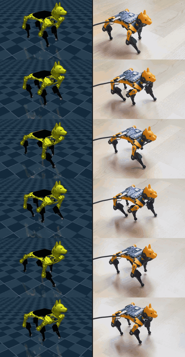
Shipped policy /cmd 0.10 m/s /left: MuJoCo /right: Bittle X @ 50 Hz
The shipped policy walking in MuJoCo on the left and on a real Bittle X on the right
One policy, one 0.10 m/s command, both sides: the gait it was trained to walk in simulation, and that same policy running on the robot.
50 Hz
Control loop
20 ms per tick, on the robot
54 ms
Command → motion
198 ms on stock firmware
0.097 m/s
Measured walk
against 0.100 commanded
2.6 %
Slew saturation
transfer gate sits at 15 %
250 Hz
IMU stream
5 Hz before the patch

Equipment data plate

Robot
Petoi Bittle X v2
alloy-geared servos
Board
BiBoard V1.0 Rev D/E
ESP32
Firmware
OpenCatEsp32 fork, B10_251121
+ realtime-mode patch
Serial link
115200 baud, ASCII
≥ 20 ms between commands
Servo response
τ = 33 ms
≤ 137 °/s, measured
Joint feedback
9.25 Hz whole-body
estimated, never measured
Policy
PPO, 512 envs, 5000 iters
trained at vx = 0.10 m/s only
Robot runtime
numpy + pyserial
no torch, no mujoco
Fitted to this hardware — a different plant needs a refit docs/measuring.md

Watch it walk first

No robot needed. This is the exact policy in deploy/policy/, running through the exact observation pipeline, action latency and actuator model it was trained against.

bash · ~3 minutes
$ git clone --recurse-submodules https://github.com/mike-grayhat/bittlejuice
$ cd bittlejuice
$ curl -LsSf https://astral.sh/uv/install.sh | sh   # if you need uv
$ uv sync

# the shipped policy, in the simulator it was trained in
$ uv run python sim/mj_eval.py -e shipped --video gait.mp4
$ uv run mjpython sim/mj_eval.py -e shipped

--video renders headless and works over SSH. Use mjpython for the interactive viewer on macOS — it ships with the mujoco wheel and is already in .venv/bin; on Linux, plain python opens the viewer.

two more worth running
$ uv run pytest                                       # the invariants, ~10 s
$ uv run python tools/mj_deployability.py -e shipped  # will this gait survive real servos?

The second is the gate that decides whether a policy transfers at all. The shipped policy reads 2.6 % slew saturation against a 15 % threshold — see docs/training.md for why that number, and not the reward curve, is the one that matters.

Ways in

Four entry points, in increasing order of effort. Each one is useful on its own, and each builds on the one above it.

Tier
You get
You need
Roughly
00
Watch the shipped policy
A laptop. No robot, no training, no GPU.
3 minutes
01
Run it on a robot
A Bittle X v2, a USB cable, and one firmware flash.
an evening
02
Train your own gait
The above, plus a decent CPU. Budget ~1.1 h per seed, and run four seeds.
+5 hours
03
Measure your own robot
The above, plus patience. Produces a plant model fitted to your hardware.
+a day

What you are working with

Three properties of this robot drive nearly every design decision. Most of what looks strange in the codebase follows from them — and the consequence is that the interesting work is in the plant model, not the algorithm. The RL is ordinary PPO.

9.25 Hzwhole-body joint read

It cannot read its joint positions

The firmware can infer one — detach the servo, turn the signal pin into an input, time a reply pulse — at roughly 20 ms a joint, with the leg limp for the duration. Against a loop that gets 20 ms per tick, that is not feedback.

So dof_pos and dof_vel are never measured. They are estimated, by replaying the host's own commanded targets through a model of the servo's measured response — and the simulator observes the same estimate rather than its own ground truth.

0raw gyro channels

It has no raw angular rate

The firmware never prints angular rates. They are finite-differenced from the fused attitude stream, and that differentiation sets the noise floor the policy has to live with.

Everything downstream — observation scaling, the disturbance model, what the reward can reasonably ask for — is drawn against that floor rather than an ideal IMU.

τ = 33 msservo step response

Its servos are slow

A naive MuJoCo actuator is much faster than the real thing, and slews well past the measured 137 °/s ceiling. Train against that and the gait will not survive contact with hardware.

The filter and the actuator have to be fitted together, or the same lag gets counted twice — which is exactly what test_actuator_dynamics.py pins.

Known & measured

It walks open-loop

Blindfold the policy — replace both IMU channels with a constant “upright and still” — and it barely notices. It loses 1.1 % of its speed, and 0.2 % on a 4° slope, the condition designed to catch a policy that reads gravity. The loop is closed in the plumbing and not in the policy: the robot is running a learned rhythm more than it is reacting to anything.

That is an open problem here, not a solved one. The most likely reason is that the policy almost never falls, so nothing ever selects for recovery. docs/training.md has what was tried and why it did not work — and the section below takes the claim as far as it goes: the whole network is reproduced by 56 numbers and a clock.

check it yourself
$ uv run python tools/blindfold_test.py -e shipped
−1.1 %
speed, blindfolded
−0.2 %
on a 4° slope
12 mm
rough terrain, no fall

The policy is a clock

Twenty-four of the thirty-three observation channels are the policy's own output handed back to it — dof_pos and dof_vel replayed from commands the host already sent, plus last_action. Of the nine that are not, three are the command, and this run pinned two of them: lin_vel_x_range: [0.1, 0.1] and lin_vel_y_range: [0, 0] were constants for all 5000 iterations. That leaves the yaw-rate channel, which the heading controller writes each step from heading error, and the six IMU channels. Freeze those and what remains is close to an autonomous dynamical system: the next action is largely a fixed function of past actions. Such a system has three possible fates — a fixed point, a limit cycle, or chaos. A walking gait is a limit cycle, and a limit cycle is a periodic function of one scalar phase. Hence: a clock.

530,323 → 56
floats to reproduce the gait
0.0960 / 0.0961
m/s — network / clock
0.8427 Hz
1.1866 s, 59.33 control steps
0.64°
fit residual, wire quantises to 1°
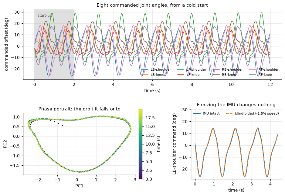
Fig 1The orbit, and the sensor it does not needclock_approximation.ipynb · §2
Top: eight commanded joint angles from a cold start, settling into a repeating pattern after about two seconds. Bottom left: a phase portrait showing a closed orbit in the first two principal components. Bottom right: the left-back shoulder command with the IMU intact and blindfolded, tracing the same waveform.
From a cold start the eight commanded joint angles settle within about two seconds, and the trace closes into a single orbit in the plane of its first two principal components — consecutive cycles then agree to 0.10°, below the 1° the command is quantised to on the wire before it reaches a servo. Bottom right is the measurement the whole reading rests on: freeze both IMU channels to “upright and still” in the current frame and all twelve history frames, and the shoulder command traces the same waveform — 0.0946 m/s against 0.0960.
Fig 2Fifty-six numbers walk the sameclock_approximation.ipynb · §5
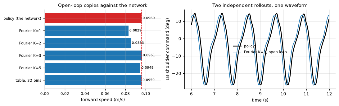
Left: forward speed by controller, with Fourier K=3 at 0.0961 m/s matching the network's 0.0960. Right: the network and the open-loop Fourier copy trace the same shoulder waveform.
Replace the actor, change nothing else. A K=3 Fourier series — 56 floats that read the wall clock and nothing else: no observation, no IMU, no last_action — walks at 0.0961 m/s against the network's 0.0960, through the same actuator lag, the same 1° wire quantisation and the same contact model. One sine per joint (24 floats) still walks, just slower and with a wider lateral wobble.

On the rough terrain the policy trained against — 20 mm heightfield, 4° slope, pushes, observation noise — three seeds put the two within noise of each other: the network averages 0.0724 m/s and falls twice on one seed, the clock averages 0.0786 m/s and does not fall. Three seeds is not a measurement, and that is the point of the open problem above: there is no evidence the network is using its sensors for anything the clock is missing.

Bring-up, off the ground first

Stock firmware cannot run this control loop — it ramps every pose command and caps the IMU at 5 Hz. The patches add a runtime mode that is off at boot, so a flashed robot still walks, dances and answers the app exactly as before until something asks. Flash with tools/flash_firmware.py: it asks the robot what it is before writing anything, refuses a mismatch, and dumps the whole flash to backups/ first, so a bad flash is one command to undo. Then bring it up in stages. Every stage is a gate.

a

Probe the link no motion

Does it talk, can it switch modes, and is the IMU stream at 250 Hz once it has?

$ uv run --directory deploy python -m bittle_io --port $PORT --run-id bringup probe
b

Dry run no serial writes

The whole policy path, with nothing reaching the servos.

$ uv run python deploy/control_loop.py --port $PORT --policy $POLICY --dry-run
c

Hold the stance pose suspended

Robot hanging, legs free. Stance pose only — no policy.

$ uv run python deploy/control_loop.py --port $PORT --policy $POLICY --hold
d

The real policy, short suspended

Still hanging. Five seconds at the commanded 0.10 m/s.

$ uv run python deploy/control_loop.py --port $PORT --policy $POLICY --command 0.10 0 0 --duration 5
e

On the floor spot it by hand

Ten seconds, spotted the first time. The policy was trained at a fixed 0.10 m/s and the export carries that range, so any other --command is clamped and the loop says so on stdout.

$ uv run python deploy/control_loop.py --port $PORT --policy $POLICY --command 0.10 0 0 --duration 10

The plant is the hardware it was fitted to. The measured plant model, the fitted servo response and the shipped policy all come from a Bittle X v2 with alloy-geared servos. Lighter plastic-geared servos and earlier revisions have their own torque and slew behaviour — read a bad gait there as a plant mismatch rather than a bad policy, and refit with docs/measuring.md. The prebuilt image on the releases page is Bittle X / BiBoard V1.0 / Rev D/E only; those are compile-time choices, so a different board needs its own build.

Where things are

deploy/ deliberately depends on nothing but numpy and pyserial — no torch, no mujoco — so it runs on limited hardware like a Pi. Copy that one directory to the robot; if you only ever want to run a policy, that is your whole install.

sim/            training pipeline: config, plant, PPO entrypoints, export
configs/        training recipes -- an objective extending a shared base
deploy/         robot runtime -- numpy + pyserial only
  bittle_io/    the measured serial layer and characterization suite
  policy/       exported policies the robot can run
tools/          diagnostics, one script per question
tests/          invariants, asserted against sim/config.py
model/          bittle.xml + meshes
logs/shipped/   the checkpoint behind the shipped policy
firmware/       submodule: the OpenCat fork, pinned to the patched branch
measurements/   hardware captures; reference/ is a full patched session
docs/           the long-form guides

How the sim is kept honest

The tests are not unit tests in the usual sense. They pin the places where sim and hardware can silently disagree, and most of them exist because that disagreement actually happened. Run them before believing anything: uv run pytest.

The fitted servo response, and that filter + actuator match the measured step response rather than double-counting ittest_actuator_dynamics.py
Sim's dof_pos/dof_vel estimate agrees bit for bit with what the deploy loop computestest_servo_observation.py
Every reward term still has usable gradient under the disturbances the environment actually appliestest_reward_support.py
Joint index and sign, against Petoi's own tabletest_joint_mapping_vs_opencat.py
The observation gets a_t while the plant gets a_{t-k}test_latency_paths.py
The loop refuses firmware that cannot switch into realtime mode, rather than walking badly against a dead IMUtest_realtime_mode.py